Fine-tuning regressions

The linear regression performed as an example on this page demonstrated that even with default settings TableTorch can produce a model with reasonable performance. However, could that performance be even better with a different configuration? Let’s find out.

We will continue using the vehicle dataset and attempt to predict value of the selling_price column.

TableTorch provides two sections of regression options: learning options impacting the regression algorithm and sampling options configuring the process of sampling the original dataset, splitting it into distinct train/test sets, as well as optionally using K-Fold Cross-Validation that performs a few regressions and automatically chooses the best model.

Let’s begin with exploring the available learning options.

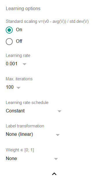
Learning options

Standard scaling: if it’s on then all the features and the label will be standard scaled before fitting the model, i.e. the regression will operate on values preprocessed with the formula

v=(v0 - average(V)) / std.dev(V)

where v0 is the original value and V is the set of all present values.

Standard scaling is a widely accepted practice for linear regressions and basically it makes sense to turn it off only if the original data has already been scaled.
Learning rate: a crucially important parameter of any gradient descent algorithm, it defines the pace at which the algorithm changes the coefficients in an effort to reach convergence. Higher values may make the regression faster but more prone to bouncing on and off certain levels. Lower values slow down the process and may even lead to a situation when the iterations count to reach convergence would be unacceptably big. As a rule of thumb, either 0.01 or 0.001 shall work well in most situations but TableTorch provides other options as well.
Max. iterations: maximum number of iterations (epochs) to perform during a regression. It usually does not make sense to change this parameter since the default of 100 is quite a high number and the regression will stop anyway once the improvement of the last few iterations is less than 1E-6 (0.000001) of relative error.
Learning rate schedule: if non-constant, decreases the learning rate accordingly after each epoch. It might allow the regression to capture ever-so-slight signal of the data.
Label transformation: if non-linear, transforms the label before learning from it. This allows to do linear regressions on labels that do not possess a linear dependency on the independent variables without introducing extra columns.

a) Exponential variant supposes that the label has an exponential dependency on the selected features and will attempt to predict a power of e rather than a linear value.

b) Logistic variant supposes that the label is in a range of [0; 1] and denotes a binary classification of a row belonging to certain class or event. It is recommended to use TableTorch’s logistic regression tool rather than this option as it will also produce a more useful summary.
Weight: if specified, then the regression uses the weighted least squares method instead of the ordinary least squares. In practice, the column that is specified as weight impacts the learning rate for each particular row and can be used to exclude or reduce influence of the outlier rows.

Let’s set the Learning transformation to Exponential and perform the regression again.

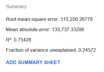
Surprisingly, both the R² and MAE metrics have improved dramatically, with R² reaching 0.75 and MAE almost halving to 136,000.

This might indicate that there’s indeed an exponential relationship between the selling_price and vehicle’s features. However, vehicle dataset lacks such features as economic inflation or accumulated vehicle depreciation rate so it might be too early to draw a conclusion regarding the nature of dependency between the vehicle’s features and the selling_price.

Let’s go back for a moment and switch the Learning transformation back to None so as to explore the sampling options.

Sampling options

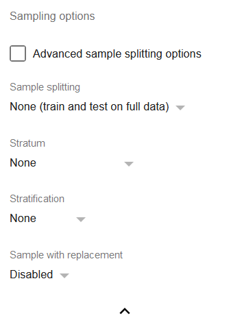
Advanced sample splitting options: check if you would like to more precisely specify train share for a train/test split or k for k-fold cross-validation.
Sample splitting: a set of the most often used dataset splitting techniques for regressions:

a) Train-test split 50/50: splits the dataset so that only 50% of the data is used for training.

b) Train-test split 80/20: same as (a) but with a higher share of data used for training.

c) 3-Fold Cross-Validation: splits the dataset into three samples A, B, and C of equal size, and then performs three different regressions, first trained on the samples (A, B) and validated on sample C, second trained on the samples (B, C) and validated on sample A, third trained on the samples (A, C) and validated on sample B, then chooses the model with the highest R².

d) 5-Fold Cross-Validation and 10-Fold Cross-Validation: generally the same as (c) but with a higher number of folds, i.e. number of regressions to perform.
Stratum: allows choosing a column identifying the stratum to which the row belongs to.
Stratification: if one of the splitting options is selected, it is possible to select one of the stratification strategies:

a) None: rows get passed into each split on a random basis.

b) Stratified proportional: each stratum is represented in each split in the same proportion that it had in the whole dataset.

c) Stratified uniform: all strata have the same number of rows in each split.
If sampling with replacement is disabled, the number of rows is determined by the number of rows in the smallest stratum. Otherwise, the number of rows is determined by the number of rows in the largest stratum. Thus, it usually makes sense to enable the replacement in case of using the stratified uniform sampling.
Sample with replacement: if enabled, each split will be sampled with replacement, i.e. there will be a probability of the same row appearing in a split twice. This is especially useful for unbalanced datasets where a particular stratum in underrepresented. With replacement, it is possible to use the random uniform stratification and avoid signal loss due to small number of rows.

Let’s do the selling_price regression again with the sample splitting option set to 3-Fold Cross-Validation.

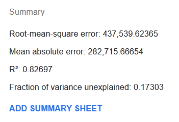
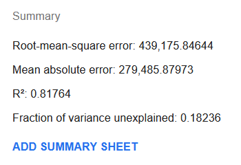
Interestingly, the R² has improved significantly reaching 0.83, whereas MAE has increased to about 283,000. This might seem confusing as it indicates that the model now probably captures the variance better even though the average absolute error has increased.

However, it shall be remembered that these results were achieved with training only on two thirds of the data. This means that this model has shown robustness against the data that it did not see during the fitting process. This is the main reason why it is a frequently used practice to do the K-Fold Cross-Validation in practically any case as it protects the model against overfitting.

Feature engineering

During the preparation process of the vehicle dataset, we’ve already modified the dataset so as to convert textual information into numeric data. However, we did not introduce any auxiliary features that could help the regression.

Furthermore, we did not pay much attention to the correlation matrix of the dataset, whereas it could be crucial to exclude highly correlated variables from the regression.

Correlation matrix tool produces the following matrix for the dataset:

The coefficients show that some of the columns can be excluded from regressing the selling_price column:

max torque max RPM due to its high correlation with max torque min RPM and negligible correlation with selling price.
petrol due to its highly significant correlation with diesel.
engine cc due to its correlation with max power bhp where the latter has higher correlation with selling_price.

Let’s deselect the columns max torque max RPM, petrol, and engine cc before doing the regression.

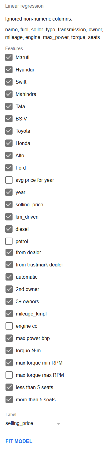
Enable the 3-Fold Cross-Validation and click Fit model to perform the regression.

The performance of the regression did neither improve nor degrade, which is a good sign: the fewer features to produce the same quality model, the better.

Now let’s try to hypothesize which additional features could be derived from the variables that are already present in such a way that would help the regression explain the variance in the label.

year stratum

If we look at the count of rows per year, it turns out that there are many years with just a few records.

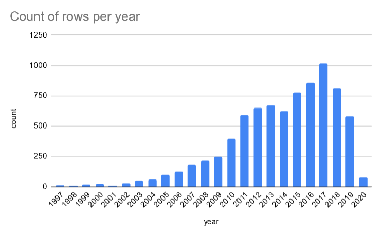
It might make sense to group the records into just a few cohorts or strata:

1-3 years (year >= 2018);
4-8 years (AND(year >= 2013, year < 2018));
9-15 years (AND(year >= 2006, year < 2013);
more than 15 years old (year < 2006).

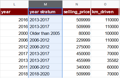
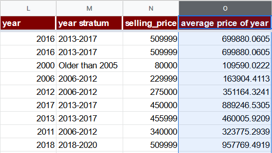
Let’s insert a column year stratum right after the year (L) column with the formula:

=IFS(L2 >= 2018, "2018-2020", L2 >= 2013, "2013-2017", L2 >= 2006, "2006-2012", TRUE, "Older than 2005")

Notice that this column has a textual value rather than a numeric one. That’s right, it won’t be used in a regression directly but will rather help with deriving other features and also used in stratified uniform random sampling.

Accounting for inflation and depreciation

Considering that vehicles have a tendency to worsen their condition with age and that the new models get ever more brilliant new features, it is reasonable to introduce a kind of an inflation + depreciation feature to gauge the average effect of these phenomena on a particular row.

One possibility of doing that would be to introduce additional data to the dataset, representing accumulated vehicle price inflation in a given year, as well as depreciation rate for a particular model. However, sometimes additional data could not be readily available or its acquisition might incur additional cost.

Hence, let’s use another option: an average price of year (O) column. Its formula will just aggregate the average price of all vehicles produced in a given year. Since there are less than 100 records per year for years lesser than 2006, for them we’ll use the average price of the “Older than 2005” stratum. Note that introduction of such a feature is a form of data leak which we will discuss later on this page.

=IF(L2 <= 2005, AVERAGEIF($M$2:$M$8129, "Older than 2005", $N$2:$N$8129), AVERAGEIF($L$2:$L$8129, L2, $N$2:$N$8129))

depreciated max power bhp (AG)

In all of the selling_price regressions that we’ve done so far, the most significant coefficient has been invariably assigned to the max power bhp feature.

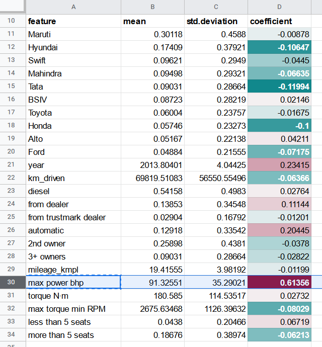
Nevertheless, as the car’s performance degrades with time, 100 bhp specification for a car produced in year 2000 may not indicate power identical to that of a car produced in 2020 with the same bhp metric.

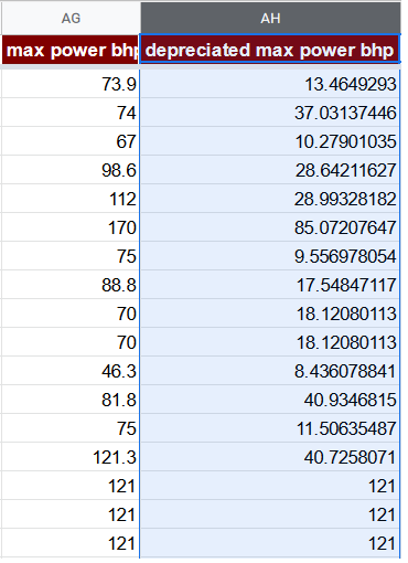
A possible way to correct the max power bhp feature in our case is to multiply it by the average price of year and then divide by the maximum average price of year. The meaning of this feature would be the perceived value of a max power bhp for a car of particular age.

=AG2 * O2 / MAX($O$2:$O$8129)

Fitting the model with new features

The correlation matrix regarding the selling_price, year and the derived features looks like this:

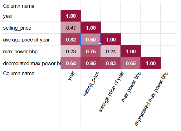
The good news is that depreciated max power bhp column has a higher correlation coefficient with selling_price than the untouched max power bhp. Furthermore, average price of year is also correlated with selling_price more significantly than the simpler year column.

Let’s add these new features into the regression while simultaneously removing columns year and max power bhp from it. The columns of max torque max RPM, petrol, and engine cc shall also be unchecked in the features list as was discussed above. Besides, the 3-Fold Cross-Validation setting should also be enabled.

Now that there’s also a year stratum column, it shall be set as a stratum column and the stratification should be set to uniform. It will ensure that each fold contains exactly the same number of rows from each stratum, reducing the model’s bias towards either newer or older vehicles.

The entire configuration of the regression is shown below.

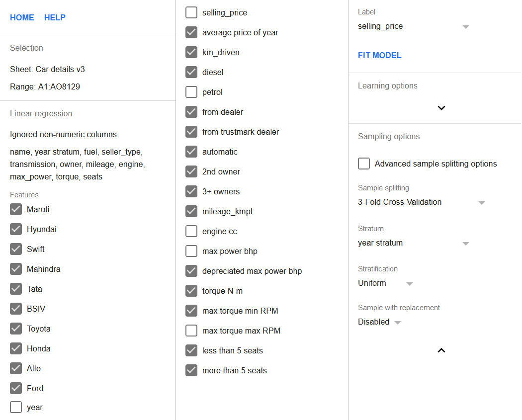
Click the Fit model button to perform the regression.

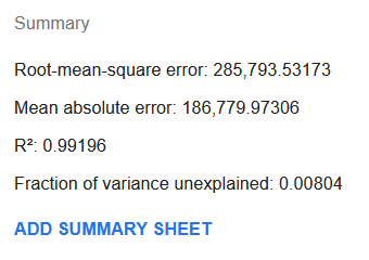
Fascinatingly, R² almost got to be as good as it could be at 0.99. Both the RMSE and MAE become significantly lower than what was the case with regression with default settings and without any derived features.

Furthermore, if we insert prediction column and relative error column =ABS((AP2 - N2) / N2) (where N is the selling_price and AP2 is the prediction) and then sort by the relative error, we can see that 19% of the rows have prediction error of 10% or less of the observed selling_price and the median relative error is around 28.8%.

Data leakage

It should be noted that deriving a feature from the dependent variable, as we did with the average price of year column, introduces a data leak. This is a situation when the label is being predicted based on the data containing itself. It can complicate or even make it impossible to use the model on the new data.

The average price of year, for example, could be moved to a separate range and for the new data we might use LOOKUP function to retrieve the value of the feature as the AVERAGEIF won’t be practical because there are no observed values for the selling_price. However, if we encounter a row having the value of year that was not observed during the training of the model, it would be impossible to find the appropriate average price of year and a best guess would need to be used instead, e.g. finding the value for the closest year.

Therefore, the improved metrics of the fine-tuned model must be appraised with caution: it might not perform as well at the prediction time if some of the derived features cannot be reliably obtained.

Conclusion

We attempted to demonstrate that the options that TableTorch provides for fine-tuning the regression process together with a bit of feature engineering can result in a more robust and reliable model than just using the default settings. There are no limits to perfection and there are more to do with modelling the vehicle dataset.

One way of improving the model might actually be in asking it a different question. For example, instead of trying to predict the precise value of the selling_price, we might try to predict whether it would sell for a price higher than certain threshold or not. TableTorch provides a suitable tool to fit a model specialized in these kind of questions, the logistic regression.

Let us know!

Thank you for using or considering to use TableTorch!

Does this page accurately and appropriately describe the function in question? Does it actually work as explained here or is there any problem? Do you have any suggestion on how we could improve?

Please let us know if you have any questions.